Correlation between income and housing characteristics in Iowa from 2005-2023
Author
Duy Doan
Published
May 30, 2025
Background
Housing affordability has become an increasingly pressing issue across the United States, with Iowa being no exception. As median home values continue to rise, understanding the relationship between household income and housing characteristics is very important.
This report examines the correlation between income and housing characteristics in Iowa from 2005 to 2023, spanning nearly two decades of economic changes including the 2008 financial crisis, its recovery, and 2020-2021 COVID Pandemic. By analyzing American Community Survey (ACS) data, we investigate how the percentage of income spent on housing has evolved over time and explore the relationship between personal earnings and housing payments.
The analysis focuses on five key research questions:
How has the percentage of household income spent on housing costs changed in Iowa from 2005 to 2023?
The changes in income compared to the median cost of a house
Ownership vs rent from 2005-2023
How do mortgage rates affect house ownership
How have major events affected the housing situation in Iowa
Understanding these trends is essential for assessing housing affordability and identifying potential policy interventions to support Iowa residents in accessing affordable housing options.
Household income growth compared to housing prices in Iowa 2005-2023
Code
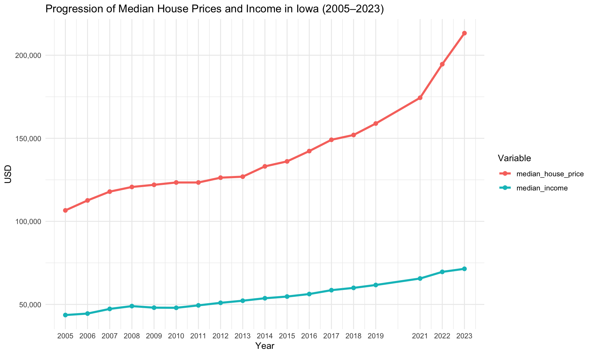
df_long <-read.csv("data/median_income_house_prices.csv")years <-c(2005:2019, 2021, 2022, 2023)ggplot(df_long, aes(x = year, y = value, color = variable)) +geom_line(linewidth =1.2) +geom_point(size =2) +scale_x_continuous(breaks = years) +scale_y_continuous(labels = comma) +labs(title ="Progression of Median House Prices and Income in Iowa (2005–2023)",x ="Year",y ="USD",color ="Variable" ) +theme_minimal()
Household income from 2005 to 2023 compared to the median house price has not kept pace with the increase in housing costs. While median household income has grown steadily over this period, median house prices have increased at a much faster rate. This is particularly evident after 2012, where house prices show exponential growth while income growth remains relatively linear. By just looking at this, we can make the \(H_0\) that houses are becoming less and less affordable.
House ownership rate
Code
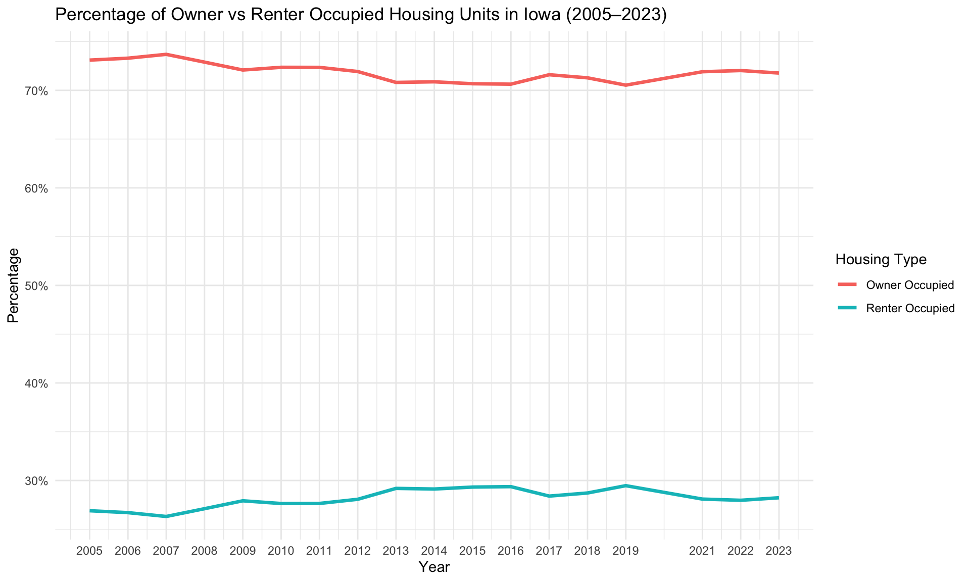
df_housing <-read.csv("data/owner_vs_renter_occupied.csv")years <-c(2005:2019, 2021, 2022, 2023)ggplot(df_housing, aes(x = year)) +geom_line(aes(y = percent_owner_occupied, color ="Owner Occupied"), linewidth =1.2) +geom_line(aes(y = percent_renter_occupied, color ="Renter Occupied"), linewidth =1.2) +scale_x_continuous(breaks = years) +scale_y_continuous(labels = scales::percent_format(scale =1)) +labs(title ="Percentage of Owner vs Renter Occupied Housing Units in Iowa (2005–2023)",x ="Year",y ="Percentage",color ="Housing Type" ) +theme_minimal()
As we can see, the housing ownership rate in Iowa has remained very stable throughout the 2005-2023 period. Despite the 2008 crisis and the COVID-19 pandemic, the percentage of owner-occupied housing units has consistently been around the 70s, while renter-occupied units have been hovering at the mid-to-high 20s. This stability suggests that major economic disruptions had minimal impact on Iowa’s overall housing trend.
The trend is further supported by research showing that Iowa has a high percentage of homeownership compared to other Midwest states and the national average, with relatively low housing costs and a low percentage of cost-burdened households (Iowa Finance Authority, n.d.).
This would seem to contradict our initial hypothesis (\(H_0\)) that houses are becoming less affordable. If housing ownership rates remain stable despite rising prices, what factors might explain this apparent contradiction and the sustained homeownership levels in Iowa?
Percentage of income spent on housing
Code
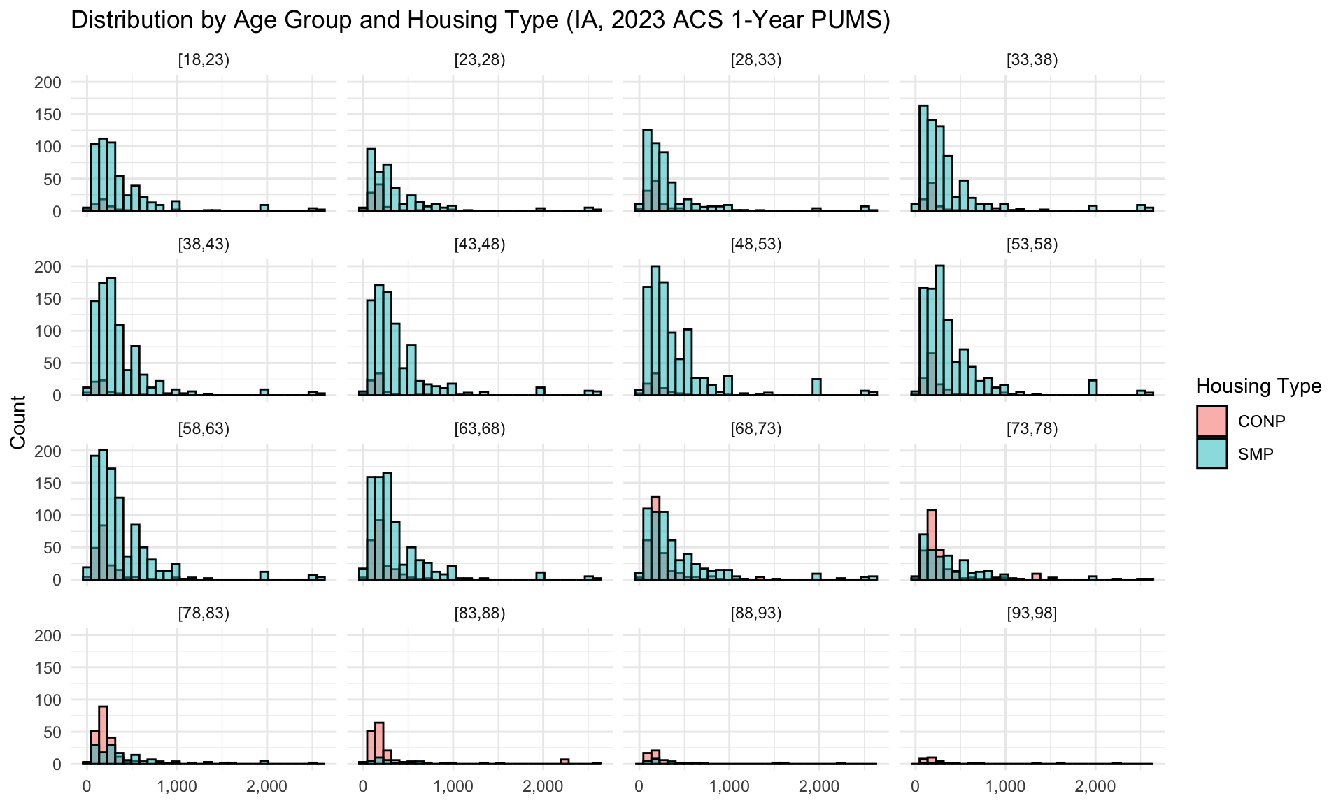
ms_3 <-read.csv("data/own_or_rent_by_age_2023.csv")ggplot(ms_3, aes(x = amount, fill = payment_type)) +geom_histogram(position ="identity", alpha =0.5, bins =30, color ="black") +facet_wrap(~ age_group) +scale_x_continuous(labels = scales::comma) +labs(title ="Distribution by Age Group and Housing Type (IA, 2023 ACS 1-Year PUMS)",x =NULL,y ="Count",fill ="Housing Type" ) +theme_minimal()
In 2023, it is evident that most people in Iowa own homes rather than rent, even among younger age groups. Ownership rates have hovered around 70% from 2005 to 2023, with little change during both the Great Recession and the COVID pandemic.
Code
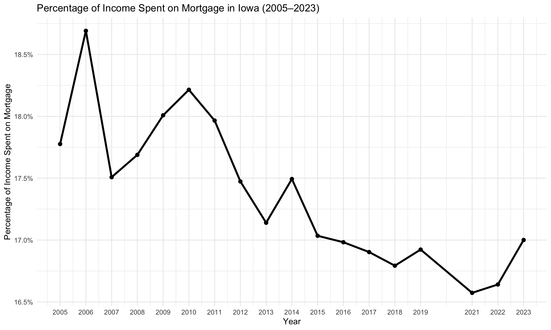
df_long1 <-read.csv("data/percent_income_spent_on_mortgage.csv")ggplot(df_long1, aes(x = year, y = percent_income_spent)) +geom_line(linewidth =1.2) +geom_point(size =2) +scale_x_continuous(breaks = years) +scale_y_continuous(labels = scales::percent_format(scale =1)) +labs(title ="Percentage of Income Spent on Mortgage in Iowa (2005–2023)",x ="Year",y ="Percentage of Income Spent on Mortgage" ) +theme_minimal()
As we can see from the data above, it is evident that people are spending less and less of their income on housing over time. This trend suggests that the growth of household income is matching or even exceeding the total cost of owning a home in Iowa. But in the previous sections, it was shown that house prices increased exponentially more than the median household income. This presents a contradiction in our analysis. So what might be the factor that correlates with Iowa’s stable house ownership rate?
Mortgage rates for the country from 1971-2025
Code
mortgage_rate <-read.csv("data/30-year-fixed-mortgage-rate-chart.csv", skip =13)mortgage_rate$date <-as.Date(mortgage_rate$date)plot_ly(mortgage_rate, x =~date, y =~value, type ='scatter', mode ='lines',name ='Mortgage Rate', line =list(color ='#1f77b4', width =2),width =1300, height =700) %>%layout(title =list(text ='National 30-Year Fixed Mortgage Rate (1971-2025)', font =list(size =18)),plot_bgcolor ='#f8f9fa', xaxis =list( title ='Year',showgrid =TRUE,gridcolor ='#e0e0e0',zeroline =FALSE), yaxis =list( title ='Rate (%)',showgrid =TRUE,gridcolor ='#e0e0e0',zeroline =FALSE),showlegend =TRUE,hovermode ='x unified')
Mortgage rates in the United States have experienced significant fluctuations from 1971 to 2025. The 2008 financial crisis led to declines, with rates dropping below 5%.
From 2008 to 2012, while the market itself was recovering, mortgage rates declined significantly, making houses more affordable.
There were slight increases between 2013-2019, but overall rates remained very stable.
However, in 2020-2021, due to the COVID pandemic, rates went as low as 2.73% after the Fed cut the federal funds rate to near zero to avoid a pandemic-induced recession (Liang and Wessel 2024).
By late 2021, it became clear that, while federal policies had shortened the pandemic recession, they had also overstimulated the economy. Inflation peaked at 9.1 percent in June 2022. The Fed responded by raising its benchmark rate sharply (Ostrowski 2025).
Comparison with similar states and bigger states
Code
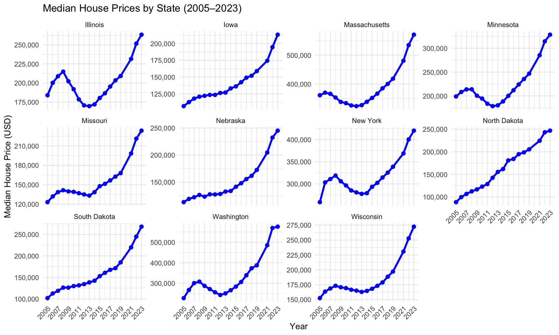
df <-read.csv("data/median_house_prices_midwest_states_and_some_big_states.csv")ggplot(df, aes(x = year, y = median_house_price)) +geom_line(linewidth =1.2, color ="blue") +geom_point(size =2, color ="blue") +facet_wrap(~ NAME, scales ="free_y") +scale_x_continuous(breaks =seq(2005, 2023, by =2)) +scale_y_continuous(labels = scales::comma) +labs(title ="Median House Prices by State (2005–2023)",x ="Year",y ="Median House Price (USD)" ) +theme_minimal() +theme(axis.text.x =element_text(angle =45, hjust =1))
Looking at the data, we can observe that larger states like New York, Washington, and Massachusetts exhibit much more dramatic price fluctuations compared to smaller Midwest states. These bigger states show steeper increases during boom periods and more pronounced dips during market corrections, while states like Iowa, North Dakota, South Dakota, and Nebraska maintain relatively steady, linear growth patterns throughout the time period.
What caused the market dips in big states?
The housing market crash of 2008-2012, fueled by the subprime mortgage crisis, saw major housing price drops across the US, with some states experiencing more severe declines than others. These price drops were primarily driven by the inability of many homeowners to repay their mortgages, leading to a surge in foreclosures and a glut of homes on the market (Weinberg, n.d.).
Why is Iowa so stable?
According to Capozza et al. (2002), “variation in the cyclical behavior of real house prices across metropolitan areas is due to more than just variation in local economies. House prices react differently to economic shocks depending on such factors as growth rates, area size, and construction costs.”
In short, what influences housing prices? Housing supply, population growth, urbanization, regulatory constraints, and interest rates (Steers Global Real Assets 2025).
Code
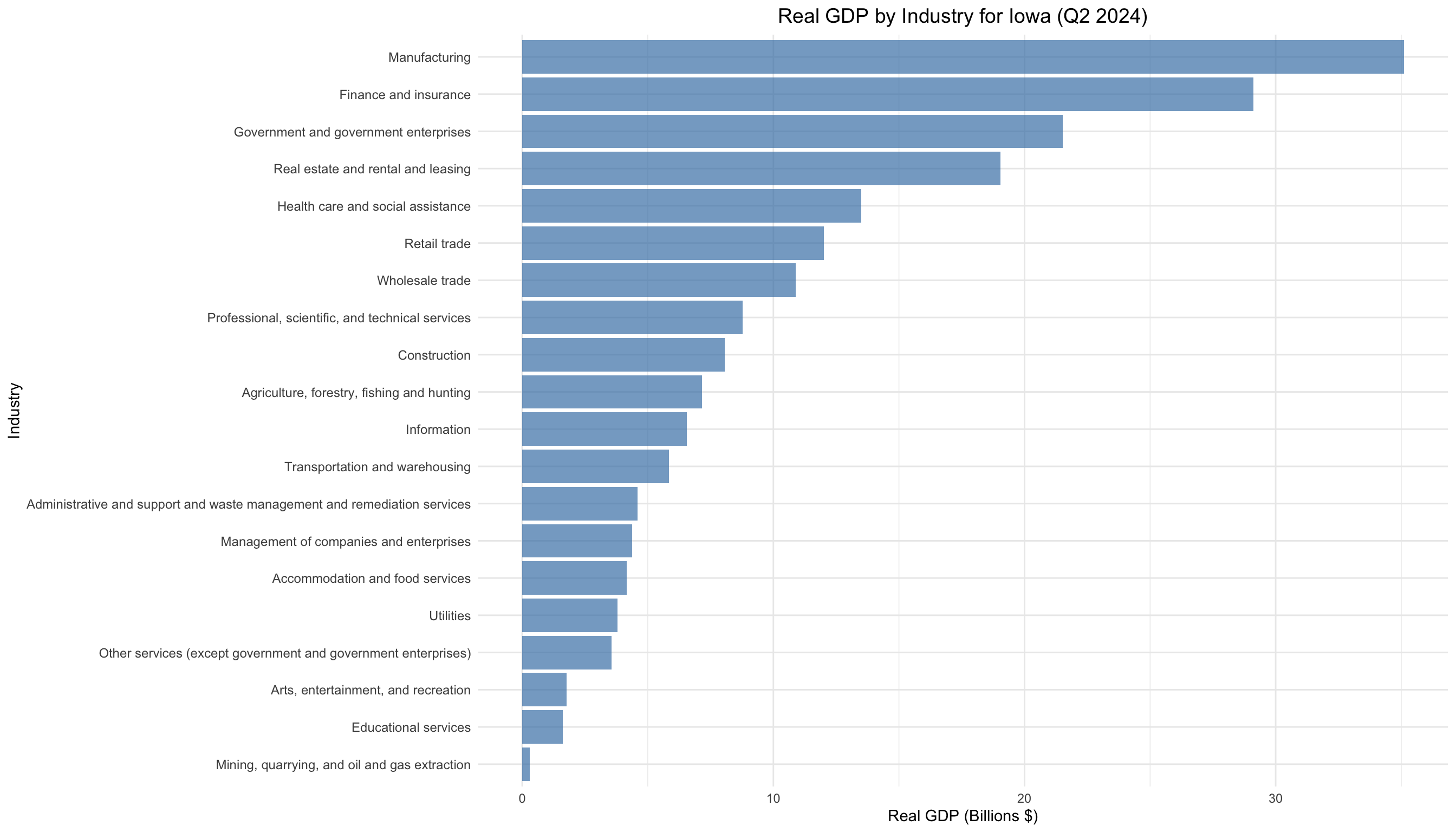
gdp <-read.csv("data/Real_GDP_for_the_State_of_Iowa__Most_Recent_Quarterly_Estimates_20250530.csv")gdp$Real.GDP.Billions <- gdp$Real.GDP /1000000000ggplot(gdp, aes(x =reorder(Industry, Real.GDP), y = Real.GDP.Billions)) +geom_col(fill ="steelblue", alpha =0.7) +coord_flip() +scale_y_continuous(labels = scales::comma) +labs(title ="Real GDP by Industry for Iowa (Q2 2024)",x ="Industry",y ="Real GDP (Billions $)" ) +theme_minimal() +theme(axis.text.y =element_text(size =9),plot.title =element_text(size =14, hjust =0.5) )
From the GDP composition chart, we can see that Iowa relies heavily on manufacturing, agriculture, and other traditional industries that provide economic stability (data.iowa.gov, n.d.). The state’s diversified economy, with significant contributions from manufacturing, finance, and agriculture sectors, creates a more resilient economic foundation that helps maintain steady housing demand without the speculative bubbles seen in tech-heavy or finance-dominated markets.
Iowa has maintained relatively stable housing prices due to several key factors: steady economic growth without dramatic booms or busts, a stable economy, lower regulatory constraints compared to coastal states, and more balanced housing supply. Additionally, Iowa’s smaller metropolitan areas and lower construction costs have contributed to this stability, making the state less susceptible to the extreme price volatility experienced in larger, more speculative housing markets.
Conclusion
The analysis shows that household income does not correlate with the rate of homeownership in Iowa, but rather that there are numerous variables in the equation. Despite disproportional growth between household income and house prices, the actual cost of owning a house has decreased significantly since 2005. It is also worth noting that Iowa’s financial growth was not heavily impacted by major financial crises. This is due to its reliance on a more stable manufacturing-based economy as shown in its GDP composition. A significant reason why it is so stable is that housing prices in Iowa are only 3 times the yearly household income, which is one of the lowest ratios in the country. In contrast, in bigger states, despite massive swings, the ratio between housing prices and income remains significantly higher.
References
Capozza, Dennis R., Patric H. Hendershott, Charlotte Mack, and Christopher J. Mayer. 2002. “Determinants of Real House Price Dynamics.” National Bureau of Economic Research. https://www.nber.org/papers/w9262.